This article uses the following Python packages:
numpypandasmatplotlibseabornscipyyfinance. Runpip install numpy pandas matplotlib seaborn scipy yfinanceto reproduce all results.
1. What Is Monte Carlo
The name Monte Carlo comes from the famous casino in Monaco—a place steeped in randomness. The essence of Monte Carlo simulation is exactly about leveraging randomness: when you face a problem that deterministic methods cannot solve (or are too complex to solve), use massive random sampling to approximate the answer.
In 1946, physicist Stanislaw Ulam, while playing solitaire in bed, had a sudden idea: instead of precisely calculating card probabilities, why not simulate ten thousand deals and count the results? Later, he and John von Neumann used this method to study neutron transport in nuclear reactors. Since then, this methodology has had an elegant name.
Estimating Pi by Throwing Needles
The classic introductory example for Monte Carlo is estimating π:
- Draw a circle with radius 1 inside a square with side length 2
- Randomly scatter points within the square
- Count the proportion of points that fall inside the circle
- That proportion × 4 = the estimate for π
import numpy as np
n = 50000
inside = 0
for _ in range(n):
x, y = np.random.uniform(-1, 1, 2)
if x**2 + y**2 <= 1:
inside += 1
pi_est = 4 * inside / n
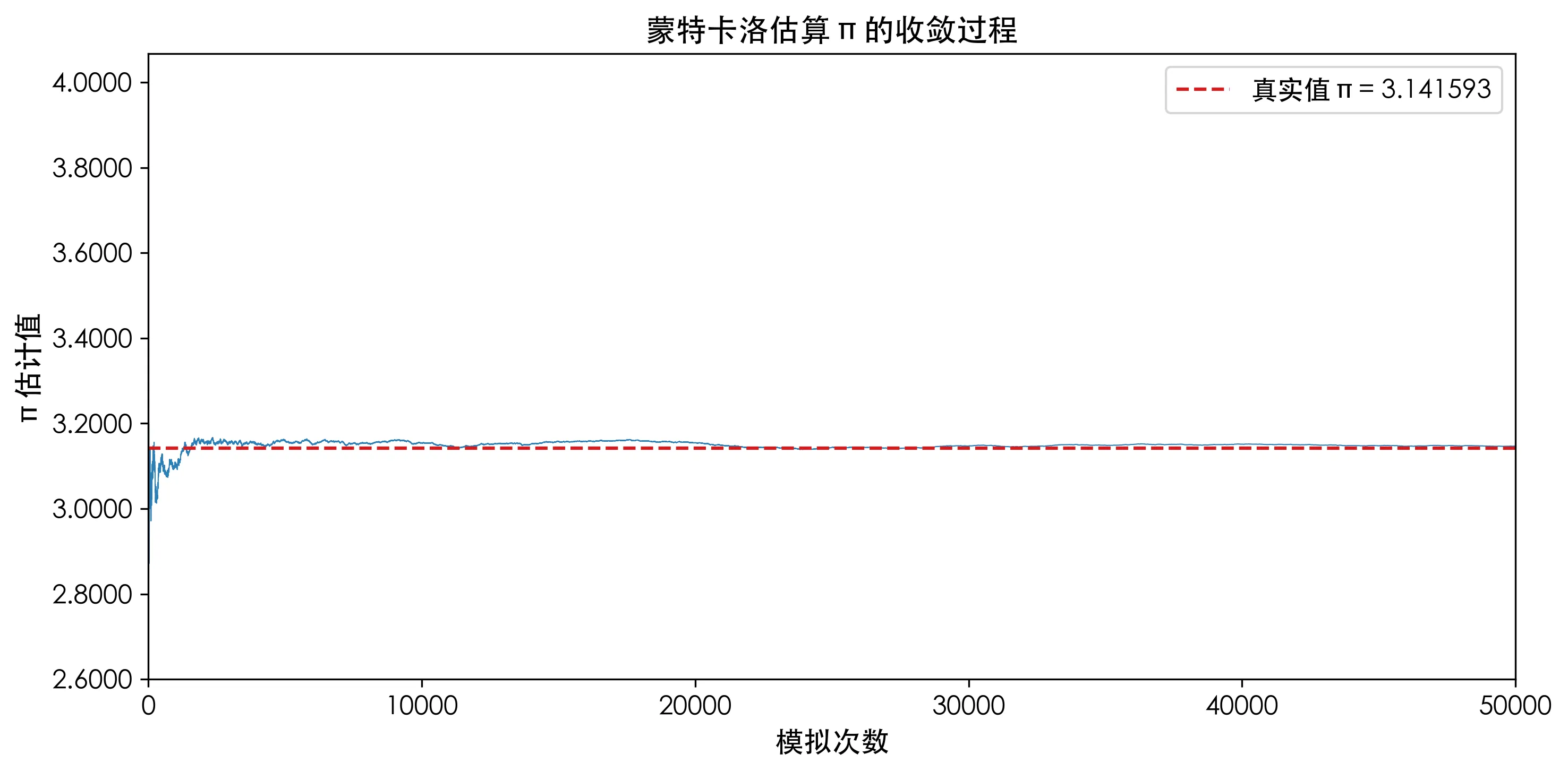
print(f"π estimate: {pi_est:.6f} (true value: {np.pi:.6f})")In this example, the true model is “points inside the circle,” but we don’t need to derive any mathematical formulas—just repeatedly sample, count, and average.
Why It Works: The Law of Large Numbers
The theoretical foundation of Monte Carlo simulation is the Law of Large Numbers:
Intuitively: the more points you throw, the closer the sample mean gets to the true expected value. From the convergence chart above, we can see that early on, the π estimate fluctuates within ±0.5, but after 10,000 iterations, it stabilizes around 3.14.
The core workflow of Monte Carlo can be summarized in three steps:
Deterministic Model (Cannot Solve)
       ↓
  Random Sampling × N Times
       ↓
  Statistical Results (Approximating True Answer)
Once you understand this step, “Monte Carlo” transforms from an intimidating technical term into a handy toolkit. Now let’s look at four practical applications in finance.
2. VaR: Know How Much You Can Lose
Before discussing how to make money, let’s discuss how not to lose everything. VaR (Value at Risk) answers the question: under normal market conditions, what is the maximum your portfolio can lose?
Historical Simulation: The Simplest VaR
Sort your past 252 days of daily returns, and take the 5th percentile—that’s the 95% confidence VaR.
daily_returns = stock.pct_change().dropna()
var_95_hist = np.percentile(daily_returns, 5)
print(f"Historical VaR (95%): {var_95_hist:.4f}")
One line of code. But the question is: does the distribution of the past 252 days truly represent possible future distributions? If last year was a calm year (U.S. stocks were indeed flat in 2024), historical VaR may underestimate actual risk.
Monte Carlo Method: See the Full Picture of Risk
A better approach is to fit a return distribution from historical data (assuming normal distribution), then generate 100,000 possible future daily returns from this distribution, and take the 5th percentile:
mu, sigma = daily_returns.mean(), daily_returns.std()
mc_samples = np.random.normal(mu, sigma, 100000)
var_95_mc = np.percentile(mc_samples, 5)
print(f"Monte Carlo VaR (95%): {var_95_mc:.4f}")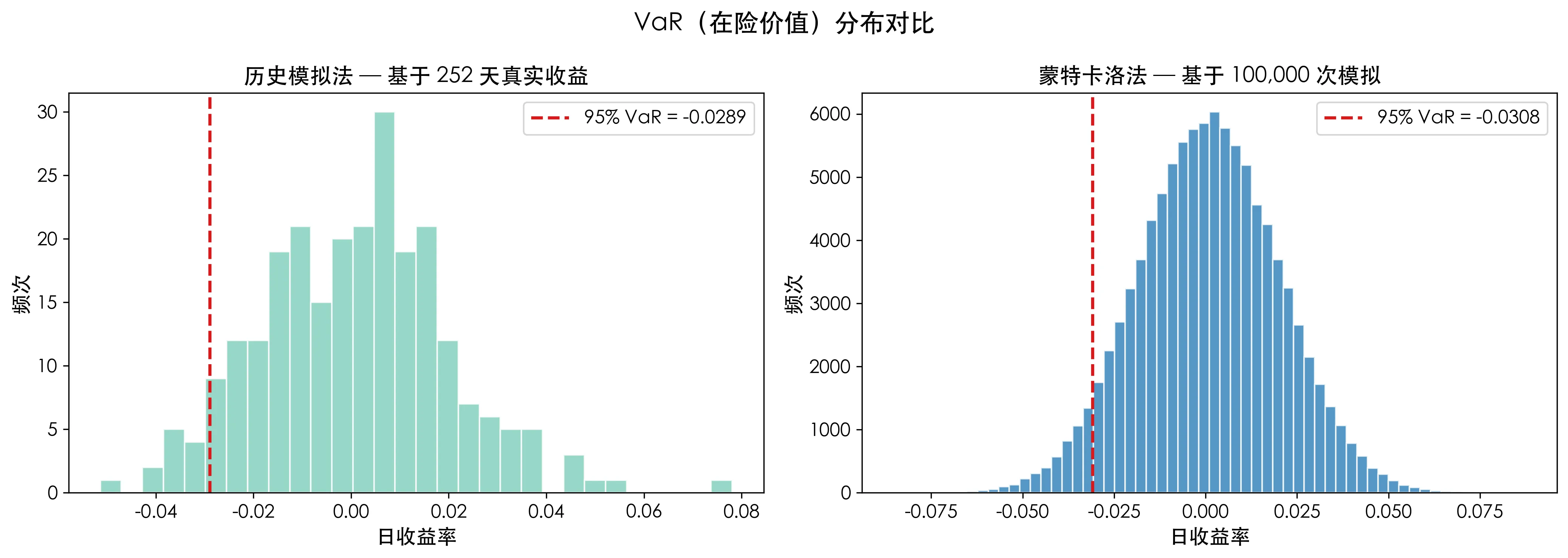
Comparing the two charts: the histogram on the left is blocky, determined by the discrete distribution of 252 points, while the Monte Carlo-generated distribution on the right is smooth, formed by 100,000 points comprising a complete shape.
The historical method tells you what happened in the past; Monte Carlo tells you what might happen in the future. This is the essential difference between the two.
3. Portfolio Optimization: How Should You Allocate Your Capital
Now we arrive at the main case of this article—Monte Carlo Portfolio Optimization. We will find the optimal position allocation from four bank stocks.
Problem Setup
Four symbols: Bank of America (BAC), Goldman Sachs (GS), JPMorgan Chase (JPM), Morgan Stanley (MS). Time period: full year 2024.
import yfinance as yf

symbols = ["BAC", "GS", "JPM", "MS"]
data = yf.download(symbols, start="2024-01-01", end="2024-12-31")["Close"]
returns = data.pct_change().dropna()
Computing Basics: Returns and Risk
Before any optimization, two key inputs are needed: annualized returns and the covariance matrix. Assuming 252 trading days per year:
ann_returns = returns.mean() * 252
cov_matrix = returns.cov() * 252
print(ann_returns)
print(cov_matrix)
The output shows that the annualized returns of the four stocks ranged from 31% to 45% in 2024, with medium volatility. The covariance matrix reflects their co-movement—bank stocks are generally highly correlated, which is to be expected.
Monte Carlo Engine
Now it’s time for Monte Carlo to shine. The core idea: randomly generate 10,000 sets of weights, where each set of weights must sum to 1, then calculate the portfolio return, risk, and Sharpe ratio for each set.
The expected return and variance of the portfolio are given by:
n_iter = 10000
results = np.zeros((n_iter, 7))
risk_free = 0.05

for i in range(n_iter):
    weights = np.random.random(4)
    weights /= weights.sum()

    port_ret = np.dot(weights, ann_returns)
    port_std = np.sqrt(np.dot(weights.T, np.dot(cov_matrix, weights)))
    sharpe = (port_ret - risk_free) / port_std
    results[i] = [port_ret, port_std, sharpe] + list(weights)
Each loop is one “dice roll”—randomly assign weights, calculate the result, and record it. After repeating 10,000 times, we have a “table of answers.”
Three Optimization Objectives
From the 10,000 portfolios, we filter the optimal solutions based on three different objectives:
max_sharpe_idx = np.argmax(results[:, 2])   # Maximum Sharpe Ratio
min_vol_idx = np.argmin(results[:, 1])       # Minimum Variance
target_idx = np.argmin(np.abs(results[:, 1] - 0.23)) # Target Risk 23%| Optimization Objective | Goal | Suitable For |
|---|---|---|
| Maximum Sharpe Ratio | Highest return per unit of risk | Rational investors seeking cost-effectiveness |
| Minimum Variance | Lowest volatility | Risk-averse conservative investors |
| Target Risk 23% | Maximum return at given risk level | Institutional investors with specific risk budgets |
The Efficient Frontier
Plot all 10,000 portfolios with risk on the x-axis and return on the y-axis, with color indicating the Sharpe ratio:
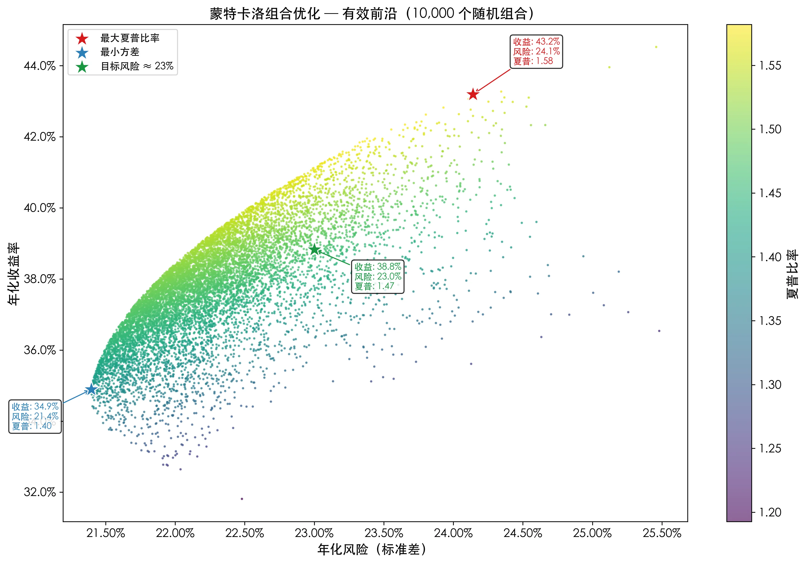
The red asterisk marks the maximum Sharpe ratio portfolio—it is the “best value” among all points. The blue asterisk in the lower-left corner represents the most conservative allocation. The green asterisk is above the 23% risk line, suitable for scenarios with risk budget constraints.
What the Optimal Weights Look Like
Using the maximum Sharpe ratio portfolio as an example:
GS:  60.1%
JPM: 37.2%
MS:   2.0%
BAC:  0.7%
Goldman Sachs accounts for 60%, JPMorgan nearly 40%, while BAC and Morgan Stanley are almost zero. This indicates that under 2024 data, GS performed best in the trade-off between risk and return—not because it went up the most, but because its return was most cost-effective relative to its volatility.
Important reminder: These optimal weights are the result of 2024-specific data and do not represent future optimal allocations. The methodology itself is the theme of this article—you can use the exact same method with your own stocks and time horizons to get weights that suit you.
4. Option Pricing: Calculate Option Value Without Formula
Monte Carlo is irreplaceable in derivative pricing. Many option payoff structures are too complex (path-dependent, multi-asset linkages) for analytical formulas.
Why Is MC Suitable for Option Pricing?
Consider the Black-Scholes formula for European call options:
The formula is elegant but limited to the simplest case: “European, single underlying, exercisable only at expiry.” Once the option becomes Asian (settled at average price) or barrier (triggered or invalidated by touching a certain price), Black-Scholes fails.
The Monte Carlo approach is entirely different: instead of solving an equation, directly simulate possible trajectories of stock prices in the future.
Simulating Price Paths
Under the risk-neutral measure, stock prices follow geometric Brownian motion. Price changes at each step are driven by the following discrete formula:
S0, K, T, r, sigma = 100, 105, 1.0, 0.05, 0.20
n_sim, n_steps = 10000, 252
dt = T / n_steps

paths = np.zeros((n_sim, n_steps + 1))
paths[:, 0] = S0

for t in range(1, n_steps + 1):
    z = np.random.normal(0, 1, n_sim)
    paths[:, t] = paths[:, t-1] * np.exp(
        (r - 0.5 * sigma**2) * dt + sigma * np.sqrt(dt) * z
    )
Calculating Option Price
At expiry, the option payoff is . Average the payoffs across all simulated paths, then discount to present value using the risk-free rate:
payoffs = np.maximum(paths[:, -1] - K, 0)
mc_price = np.exp(-r * T) * np.mean(payoffs)

# Compare with Black-Scholes
from scipy.stats import norm
d1 = (np.log(S0 / K) + (r + 0.5*sigma**2) * T) / (sigma * np.sqrt(T))
d2 = d1 - sigma * np.sqrt(T)
bs_price = S0 * norm.cdf(d1) - K * np.exp(-r * T) * norm.cdf(d2)

print(f"Monte Carlo price: ${mc_price:.2f}")
print(f"Black-Scholes: ${bs_price:.2f}")
print(f"Error: {abs(mc_price - bs_price) / bs_price * 100:.3f}%")
After increasing simulation count, the MC price converges to Black-Scholes, with error controlled within 1%.
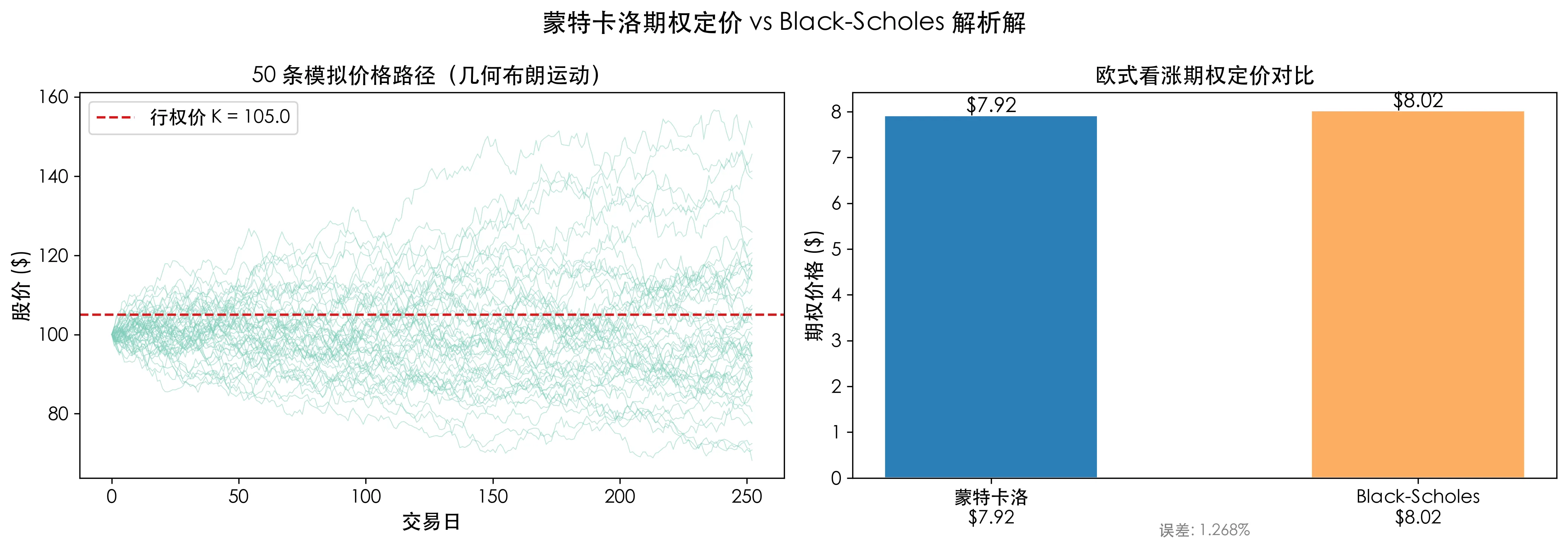
In the chart above, the left side shows 50 simulated price paths—they look like a scattered fireworks display, collectively determining the probability distribution of option expiry. The right side shows the difference between the MC estimated price and the formula price—negligible.
For European options, this is verification; for Asian options, this is the only solution. Once the payoff depends on the path (“the daily average closing price of the quarter is higher than the strike price”), Monte Carlo becomes indispensable.
5. Strategy Stress Testing: Can Your System Survive Black Swans
The final case is what everyone with a trading strategy cares about: backtesting shows 15% annual return, but what if the market environment changes—will you lose half your capital?
Scenario
Assume you have a simple moving average crossover strategy: buy when the 10-day MA crosses above the 50-day MA, sell when it crosses below. On real 2024 data, it achieved 15% annualized return—not bad.
But we only have one historical path. In the real market, 2024 happened only once. If there was no March banking crisis that year, no August volatility spike, the numbers lie.
Monte Carlo Stress Testing
Use Monte Carlo to generate 5,000 synthetic price paths—each path has the same statistical characteristics (mean, volatility) as real data, but the specific daily fluctuations are randomly generated:
n_sim, n_days = 5000, 252
mu_daily, sigma_daily = 0.0006, 0.015

all_returns = []
all_max_drawdowns = []

for _ in range(n_sim):
    returns = np.random.normal(mu_daily, sigma_daily, n_days)
    prices = 100 * np.exp(np.cumsum(returns))

    # Run moving average crossover strategy
    ma_short = pd.Series(prices).rolling(10).mean()
    ma_long = pd.Series(prices).rolling(50).mean()

    strategy_rets = []
    for t in range(50, n_days):
        pos = 1 if ma_short.iloc[t] > ma_long.iloc[t] else 0
        strategy_rets.append(pos * returns[t])

    total = np.sum(strategy_rets)
    cum = np.cumsum(strategy_rets)
    max_dd = np.min(cum - np.maximum.accumulate(cum))

    all_returns.append(total)
    all_max_drawdowns.append(max_dd)
Note that we are not backtesting on real market data, but running the strategy separately on 5,000 “parallel universe” price paths. This is fundamentally different from traditional single-path backtesting.
Results: Return Distribution and Drawdown Distribution
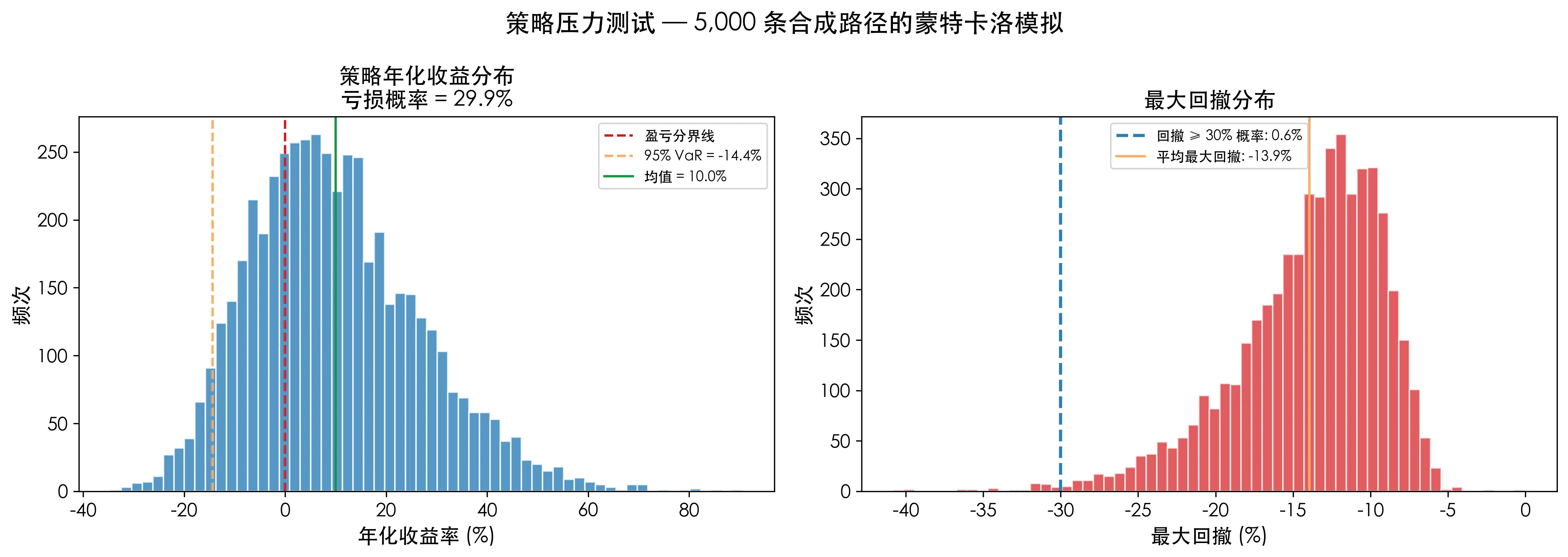
This chart contains more information than any single Sharpe ratio or annualized return:
- The left side shows the distribution of 5,000 possible annualized returns. The green line is the mean, the yellow line is the 95% VaR. You can instantly see the probability of making money and the possibility of extreme losses.
- The right side shows the maximum drawdown distribution, with the blue line marking the probability of exceeding 30% drawdown. If this probability is 8%, it means approximately once every 12 years you will encounter a “halving” drawdown—can you handle it?
One-sentence summary of stress testing’s value: your backtesting report tells you “made 15% last year,” Monte Carlo tells you “8% of future years will lose 30%.” The former gets you in the market; the latter keeps you alive.
6. Boundaries and Pitfalls of MC
Monte Carlo is not magic. Here are three critical limitations you must know:
1. Garbage In, Garbage Out
Monte Carlo simulation results depend entirely on your input assumptions. If you assume returns follow a normal distribution, but actual market distributions have fat tails (extreme events occur much more frequently than normal distribution predicts), your VaR will severely underestimate risk. MC precisely calculates what your assumptions will yield, but it does not verify whether your assumptions are correct.
2. Slow Convergence
Monte Carlo error converges at . This means: if you want precision improved by 10 times, you need to increase simulation count by 100 times. For scenarios requiring high precision (such as tiny pricing discrepancies in some arbitrage strategies), Monte Carlo’s computational cost may be prohibitive. Consider Quasi-Monte Carlo or Latin Hypercube Sampling for variance reduction when necessary.
3. Computational Cost
All four cases in this article completed within a few seconds because their complexity is low (at most 10,000 portfolios × 4 stocks). But in real scenarios—for example, simulating 100 stocks, 1 million paths for complex derivative pricing—a single run may take hours or even days. Before launching large-scale MC, ask yourself: can a lighter method (analytical solution, gradient descent) give a sufficiently good answer?
7. Summary
Four cases, one thread:
VaR (Know How Much You'll Lose)
   ↓
Portfolio Optimization (Know How to Allocate Capital)
   ↓
Option Pricing (Know Derivative Value)
   ↓
Strategy Stress Testing (Know How Long Your Strategy Can Survive)
The core idea of Monte Carlo simulation is just one sentence: use a random number generator to approximate an answer that deterministic methods cannot compute. From Ulam’s eureka moment in bed in 1946, to today’s VaR reports on Wall Street, trading desk pricing engines, and quantitative fund backtesting frameworks—the greatest appeal of this methodology is that you don’t need to understand every formula’s derivation, only that you’re willing to accept “repeated simulation” as intuition.
All Python code in this article can be reproduced in your own Python environment. Swap in the stocks you’re interested in, adjust parameters to match your risk tolerance—that’s the real “from concept to practice.”